Original English dissertation · scientific equations reproduced directly from the source PDF.

3 Experimental Methods

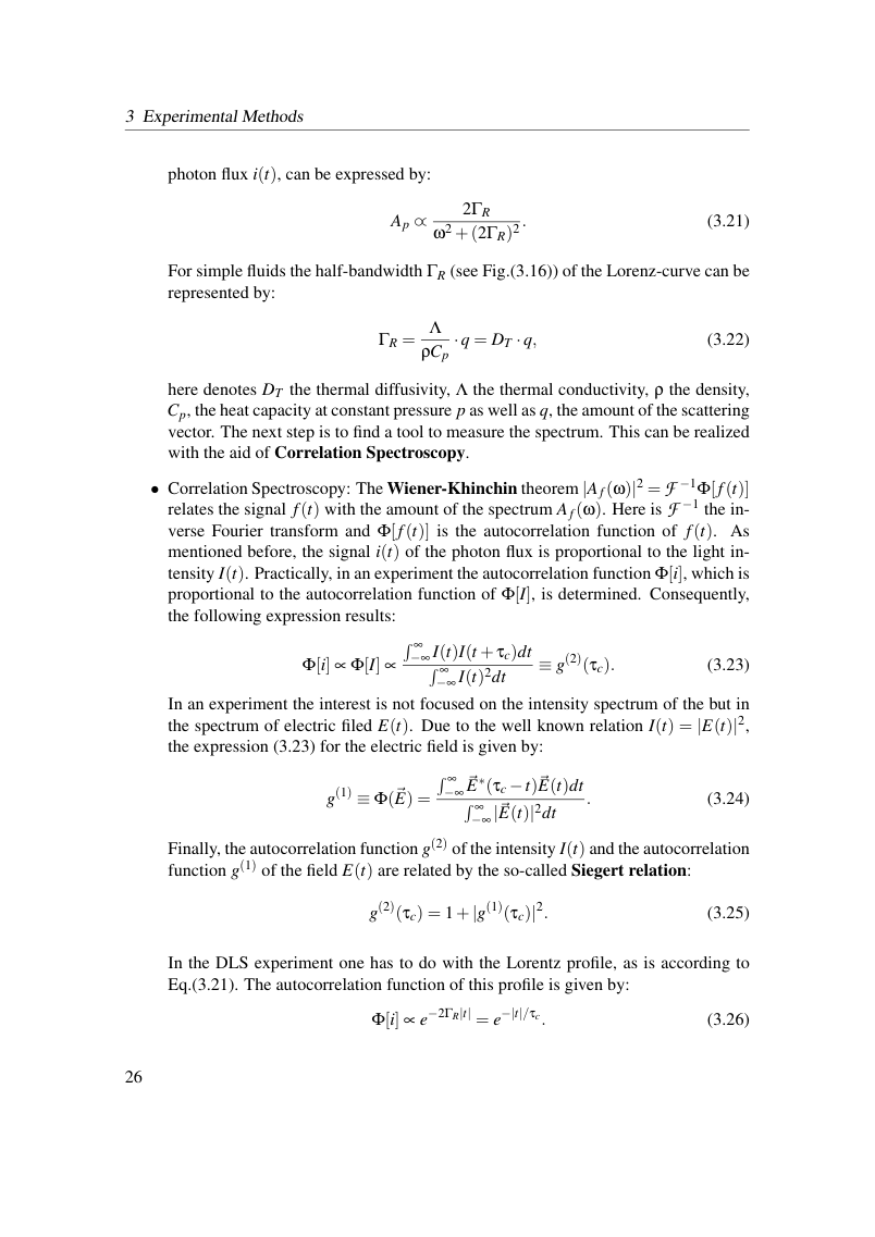
photon flux i(t), can be expressed by:

For simple fluids the half-bandwidth ΓR (see Fig.(3.16)) of the Lorenz-curve can be represented by:

here denotes DT the thermal diffusivity, Λ the thermal conductivity, ρ the density, Cp, the heat capacity at constant pressure p as well as q, the amount of the scattering vector. The next step is to find a tool to measure the spectrum. This can be realized with the aid of Correlation Spectroscopy.

• Correlation Spectroscopy: The Wiener-Khinchin theorem |Af (ω)|2 = F −1Φ[f(t)] relates the signal f(t) with the amount of the spectrum A f (ω). Here is F −1 the in- verse Fourier transform and Φ[f(t)] is the autocorrelation function of f(t). As mentioned before, the signal i(t) of the photon flux is proportional to the light in- tensity I(t). Practically, in an experiment the autocorrelation function Φ[i], which is proportional to the autocorrelation function of Φ[I], is determined. Consequently, the following expression results:

In an experiment the interest is not focused on the intensity spectrum of the but in the spectrum of electric filed E(t). Due to the well known relation I(t) = |E(t)|2, the expression (3.23) for the electric field is given by:

Finally, the autocorrelation function g(2) of the intensity I(t) and the autocorrelation function g(1) of the field E(t) are related by the so-called Siegert relation:

In the DLS experiment one has to do with the Lorentz profile, as is according to Eq.(3.21). The autocorrelation function of this profile is given by:

View original page 32 (authoritative equations, figures and layout)